hIPPyMFEM
Deterministic and Bayesian inverse problems on MFEM, with differentiable physics.
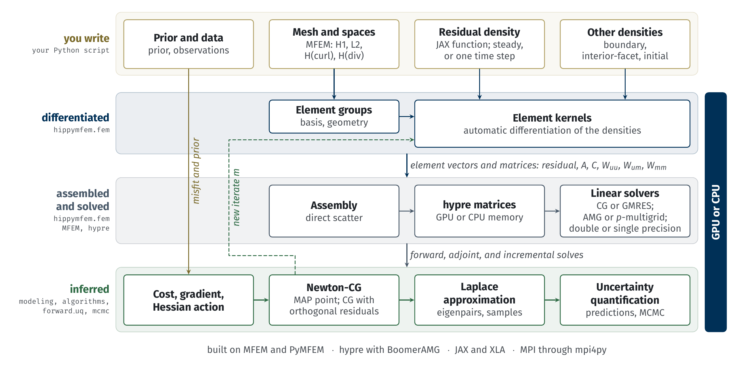
hIPPyMFEM is a library for inverse problems governed by PDEs, built on MFEM, hypre and JAX. You write the weak residual of the forward PDE once, as a density at a single quadrature point, and the library supplies everything a PDE-constrained inverse problem needs:
adjoint-based gradients and matrix-free reduced Hessians, exact for the discretized problem rather than approximated;
inexact Newton-CG (line search and trust region) for the MAP point, and limited-memory BFGS as an independent check;
a low-rank Laplace approximation of the posterior from randomized generalized eigensolvers;
Matern-class (bi-Laplacian) priors with exact sampling;
dimension-independent MCMC (pCN, gpCN, MALA) and forward uncertainty propagation;
in parallel over MPI, on MFEM meshes and finite element spaces. The element kernels run on a GPU when one is asked for, and with a CUDA or HIP build of PyMFEM the matrices and the solves do as well, which is where the large factors are (see Running on a GPU).
import mfem.par as mfem, jax.numpy as jnp
from mpi4py import MPI
import hippymfem as hm

mfem.Hypre.Init()
mesh = mfem.ParMesh(MPI.COMM_WORLD,
                    mfem.Mesh.MakeCartesian2D(48, 48, mfem.Element.TRIANGLE))
Vu, Vm = hm.FunctionSpace.H1(mesh, 2), hm.FunctionSpace.H1(mesh, 1)

def pde_varf(u, m, p, x):            # the weak residual, pointwise
    return jnp.exp(m.val) * hm.inner(u.grad, p.grad)

bc = hm.DirichletBC(Vu, lambda x: x[1], bdr_attributes=[1, 3])
pde = hm.PDEVariationalProblem([Vu, Vm, Vu], pde_varf, bc, bc.homogeneous(),
                               is_fwd_linear=True)
Nothing else about the forward problem has to be written down: the adjoint operator, the parameter Jacobian, the second-order blocks of the Lagrangian and even third derivatives are obtained by differentiating that one density.
Why differentiate a program
Libraries built on a form language, such as the FEniCS-based
hIPPYlib, obtain these operators by applying
ufl.derivative to a UFL form. MFEM has no form language, so hIPPyMFEM
differentiates the pointwise residual density at quadrature points with JAX
instead, and hands the resulting element arrays to a direct scatter into the parallel
matrix. Three consequences follow, and they are the reason the library exists:
The density is ordinary Python. Anything JAX can differentiate is a valid residual, including things no form language can express: a neural network closure, a table lookup, an inner Newton solve for a local constitutive law. The derivatives stay exact.
The kernels can run on a GPU without the residual being rewritten, because they are JAX programs rather than generated C.
Every block comes from one differentiation of one object, so the gradient and Hessian are consistent with each other and with the same quadrature rule by construction, not by agreement between separately generated kernels.
The cost is stated as plainly: see Limits, stated up front. The inverse-problem classes keep hIPPYlib’s interface conventions, so scripts written for it port with few changes (Coming from hIPPYlib).
User guide
- Installation
- Concepts
- Finite element spaces
- Boundary terms
- Interior facet terms and DG
- Priors
- Observations and misfits
- Linear solvers
- Finding the MAP point
- The posterior
- MCMC
- Forward uncertainty propagation
- Time-dependent problems
- Running on a GPU
- Configuration
- Performance
- Parallel correctness
- An application: basin-scale geothermal inversion
Tutorials
- MFEM101: solving a PDE with hIPPyMFEM
- Coefficient field inversion in an elliptic partial differential equation
- Bayesian quantification of parameter uncertainty
- Bayesian initial condition inversion in an advection-diffusion problem
- Spectrum of the preconditioned Hessian misfit operator
- Sampling the posterior with MCMC
- Gaussian priors in infinite dimensions
- Residuals as programs: a law no form language can write
- On the GPU: the same script, different hardware
- Densities on faces: discontinuous Galerkin
- Vector fields and mixed systems
- Predicting a number, not a field
Project